Simulating Phase Transitions: Building a 2D Ising Model in TypeScript
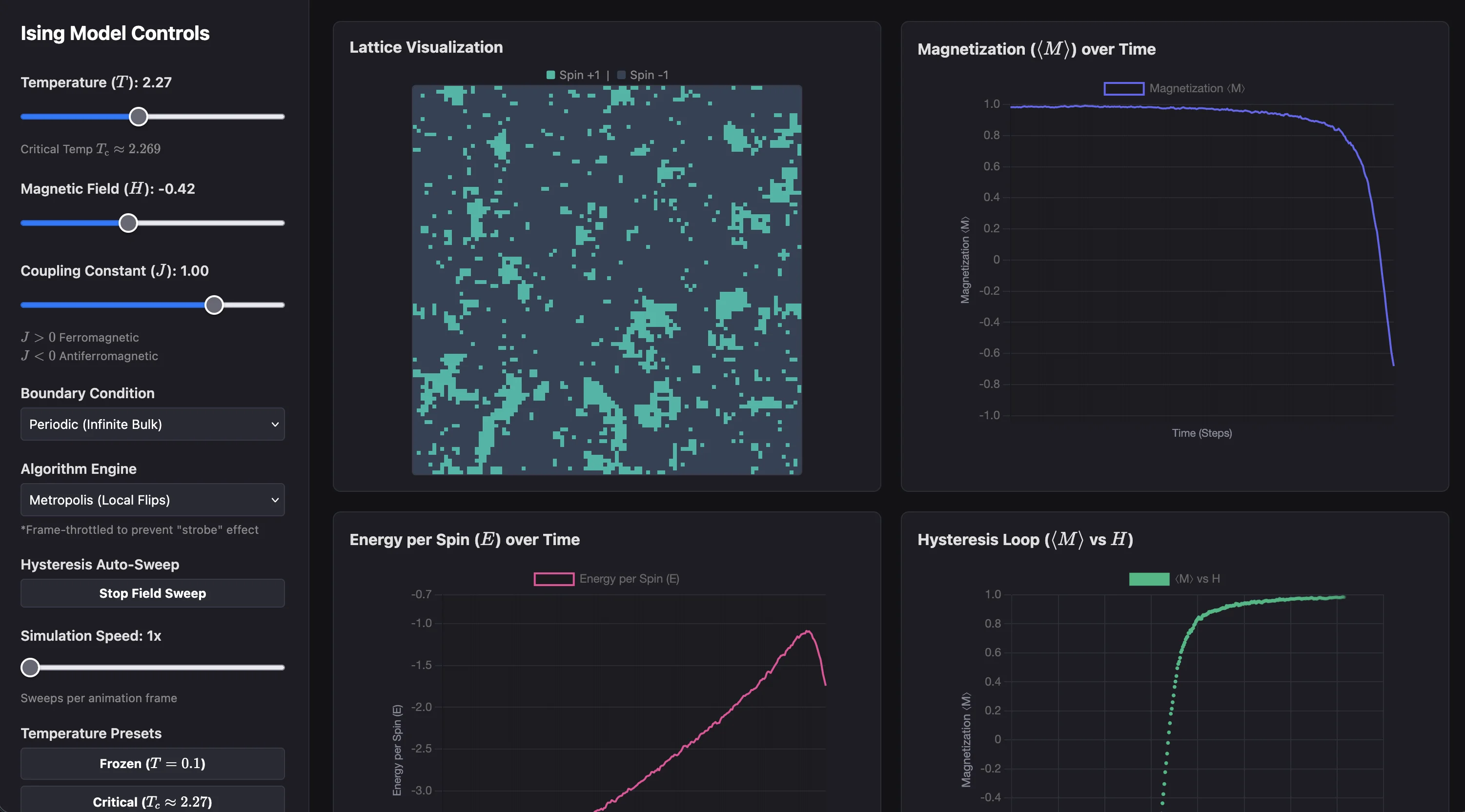
The blog post regarding a web-deployed 2D Ising model simulation, written in TypeScript, HTML 5 Canvas, and Chart.js.
In statistical physics, few models are as elegant or insightful as the Ising Model. Originally proposed by Wilhelm Lenz and solved in 1D by his student Ernst Ising in 1925, it serves as a simple mathematical abstraction for ferromagnetism.
To better visualize critical phenomena and phase transitions, I built a real-time 2D Ising Model simulation using TypeScript, HTML5 Canvas, and Chart.js.
👉 Try the Live Interactive Simulation Here
The Physics Behind the Simulation
The 2D Ising model consists of a square lattice of discrete variables called spins, where each spin \(s_i\) can take a value of either \(+1\) (spin up) or \(-1\) (spin down).
The Hamiltonian
The total energy \(E\) of the system is governed by the Hamiltonian \(\mathcal{H}\): \[\mathcal{H}(\sigma) = -J \sum_{\langle i, j\rangle} s_i s_j - H\sum_{i} s_i,\]
Where:
- \(J\) is the coupling constant (\(J > 0\) models ferromagnetism, encouraging adjacent spins to align).
- \(\langle i, j\rangle\) represents summation over nearest-neighbor lattice pairs.
- \(H\) is the external magnetic field attempting to align spins in a preferred direction.
Order Parameter: Magnetization (\(\langle M \rangle\))
The primary quantity used to measure the global order of the lattice is the mean magnetization per spin, \(\langle M \rangle\): \[\langle M \rangle = \frac{1}{N} \sum_{i=1}^{N} s_i,\]
Where \(N = L \times L\) is the total number of spins in the lattice.
- \(\langle M \rangle = +1\) represents total spin-up saturation.
- \(\langle M \rangle = -1\) represents total spin-down saturation.
- \(\langle M \rangle \approx 0\) indicates a disordered state with equal populations of up and down spins.
Phase Transitions and Critical Temperature (\(T_{\rm c}\))
In two dimensions, Lars Onsager famously showed that the Ising model exhibits a second-order phase transition at a specific critical temperature \(T_{\rm c}\): \[T_{\rm c} = \frac{2J}{k_{\rm B} \ln{\left(1+\sqrt{2}\right)}} \approx 2.269 \frac{J}{k_{\rm B}}.\]
- Below \(T_{\rm c}\) (\(T < T_{\rm c}\)): Spontaneous symmetry breaking occurs. The system aligns into large domain blocks of up or down spins, yielding a nonzero net magnetization \(\langle M \rangle \neq 0\).
- Above \(T_{\rm c}\) (\(T > T_{\rm c}\)): Thermal fluctuations overcome coupling energy \(J\), destroying long-range order and driving \(\langle M \rangle \to 0\).
Boundary Conditions
To study finite-size scaling and edge effects, the simulation allows swapping between three distinct boundary conditions:
- Periodic Boundary Conditions (PBCs): The top and bottom edges connect to each other, as do the left and right edges, embedding the \(2\text{D}\) lattice onto a torus. This eliminates surface effects entirely, accurately approximating an infinite bulk material: \(\text{Right Neighbor of } (L-1, y) \to (0, y).\)
- Open Boundary Conditions (OBCs): Spins along the perimeter have fewer nearest neighbors (\(3\) on edges, \(2\) at corners). This introduces physical surface tension and surface relaxation phenomena.
- Fixed Boundary Conditions: The perimeter spins are locked into a fixed orientation (e.g., all \(+1\) or all \(-1\)). This acts as a constant external boundary field, forcing domain formation even at elevated temperatures.
Algorithms: Local vs. Cluster Updates
The simulation supports two distinct Monte Carlo sampling algorithms to highlight how computational efficiency changes near critical points:
1. Metropolis-Hastings Algorithm (Local Updates)
At each step, a single spin \(s_i \to -s_i\) is randomly selected and evaluated based on the change in energy \(\Delta E\):
- If \(\Delta E \le 0\), the flip is accepted immediately.
- If \(\Delta E > 0\), the flip is accepted with Boltzmann probability \(P = e^{-\Delta E / k_{\rm B} T}\).
- Use Case: Excellent for observing non-equilibrium time evolution, domain nucleation, and magnetic hysteresis under a dynamic external field \(H\).
- Limitation: Suffers from critical slowing down near \(T_{\rm c}\), where local updates struggle to flip large, correlated clusters.
2. The Wolff Cluster Algorithm (Global Updates)
To circumvent critical slowing down near \(T_{\rm c}\), the Wolff algorithm identifies and flips entire clusters of aligned spins simultaneously:
- Select a random seed spin \(s_i\).
- Recursively add like-minded nearest neighbors (\(s_j = s_i\)) to the cluster with bond addition probability: \(P_{\text{bond}} = 1 - e^{-2J / k_{\rm B} T}.\)
- Invert every spin within the constructed cluster in a single step.
- Use Case: Drastically reduces correlation time near \(T_{\rm c}\), allowing the lattice to reach thermal equilibrium exponentially faster than single-spin flips.
- Note: In the live deployment, the frame limit of the Wolff flips are throttled. This is to prevent the strobe-like appearance of the large flips when they occur.
Performance & Real-Time Visualization
Simulation Speed & Monte Carlo Steps (MCS)
To benchmark performance independent of grid size, time is measured in Monte Carlo Steps (MCS). One MCS represents \(N\) individual spin update attempts, giving every spin on the lattice a statistical opportunity to flip once.
To achieve smooth 60 FPS performance in single-threaded JavaScript/TypeScript:
- Flat Array Layout: Spins are stored in a contiguous 1D
Int8Array(y * L + x) to maximize CPU cache locality. - Precomputed Boltzmann Factors: Acceptance probabilities for all possible local energy states (\(\Delta E \in \{4J, 8J\}\)) are precomputed into a lookup array, eliminating runtime calls to
Math.exp().
Real-Time Diagnostics & Hysteresis Graphs
The application includes three synchronized real-time plots powered by Chart.js:
- Magnetization Time Series (\(\langle M \rangle\) vs. Time): Tracks real-time fluctuations in global spin alignment.
- Energy per Spin Time Series (\(E\) vs. Time): Monitors total system energy relaxation towards thermal equilibrium.
- Dynamic Hysteresis Loop (\(\langle M \rangle\) vs. \(H\)): When sweeping the external field \(H\), the magnetization lags behind the field, tracing out a closed hysteresis loop. To make the direction of traversal clear on screen, points are drawn using a high-density scatter array with a time-faded opacity trail.
Accessible Design Choices
Default red/green spin representations can be difficult to distinguish for users with color-vision deficiencies (red-green color blindness, etc.). The lattice instead uses a high-contrast palette of dark slate and emerald teal, paired with math labels powered by KaTeX typesetting.
Try It Out
You can adjust temperature, external fields, boundary conditions, and sweep speeds interactively on the project page:
Note that the simulation dashboard is neither optimized nor currently designed for mobile viewing.
