Kapitza Pendulum Analysis
The following project involves the numerical analysis and manim animation of a Kapitza pendulum system as a part of a theoretical mechanics course final project. Specifically, we use Manim animations and Hopf bifurcation analysis to inspect the stability of the inverted position of the pendulum in the high-driving, low-amplitude regime. This is done with a mix of analytical and numerical methods.
Overview
It would be a great disservice to restate everything this project completes in this project post. Not only would the post be too long and dense to have a pleasurable reading experience, the Project notebook file already provides a comprehensive step-by-step breakdown of the project, written to be a self-contained lesson. Inspecting the various .py files shows the different numerical solving methods used to solve this system.
Briefly, this project does the following:
- Derives the Lagrangian, equations of motion, and effective potential for the Kapitza pendulum system, while inspecting the high-driving, low-amplitude regime.
- Implements numerical methods to solve the system and check that turning off the driving components recovers the simple pendulum.
- Dynamic widget analysis of the system with varying parameters.
- \(U(\phi,t)\) and \(U_{\rm eff}(\phi)\) comparisons for high-driving, low-amplitude regime, with separate PDF derivation.
- Manim animations of the system, with normalized state space axis as well.
- Chaos and bifurcation analysis: using Liapunov exponent to judge chaos. Manim animations of two pendula for chaos, with animated Liapunov exponent graph. Hopf bifurcation discrete analysis with checks on stability vs. instability of the vertical position using the bifurcation plot. Further analysis on the low-amplitude area, showing periodic motion but no chaos.
Included in the Github repository:
- All project files: the project Jupyter notebook, the PDF derivation file, any
.pynumerical files, and the outputted images. - The Conda environment used for the project, built for M-architecture OS.
- The presentation file given as a part of this project.
Manim animations are hosted in the releases, as they are big, hosted in the
videos.zipfile in each release description. Two examples are shown below, but in order to get it to display, it has been converted to a gif, which greatly reduces its overall quality. It is recommended to download the zip for higher-fidelity animations. The zip file is here.
An example (low-quality) animation of a stable vertical-position oscillation of the Kapitza system.
An example (low-quality) chaos animation of a Kapitza system with two superimposed oscillators and the Lyapunov exponent.
The System
This is the Kapitza system we wish to solve:
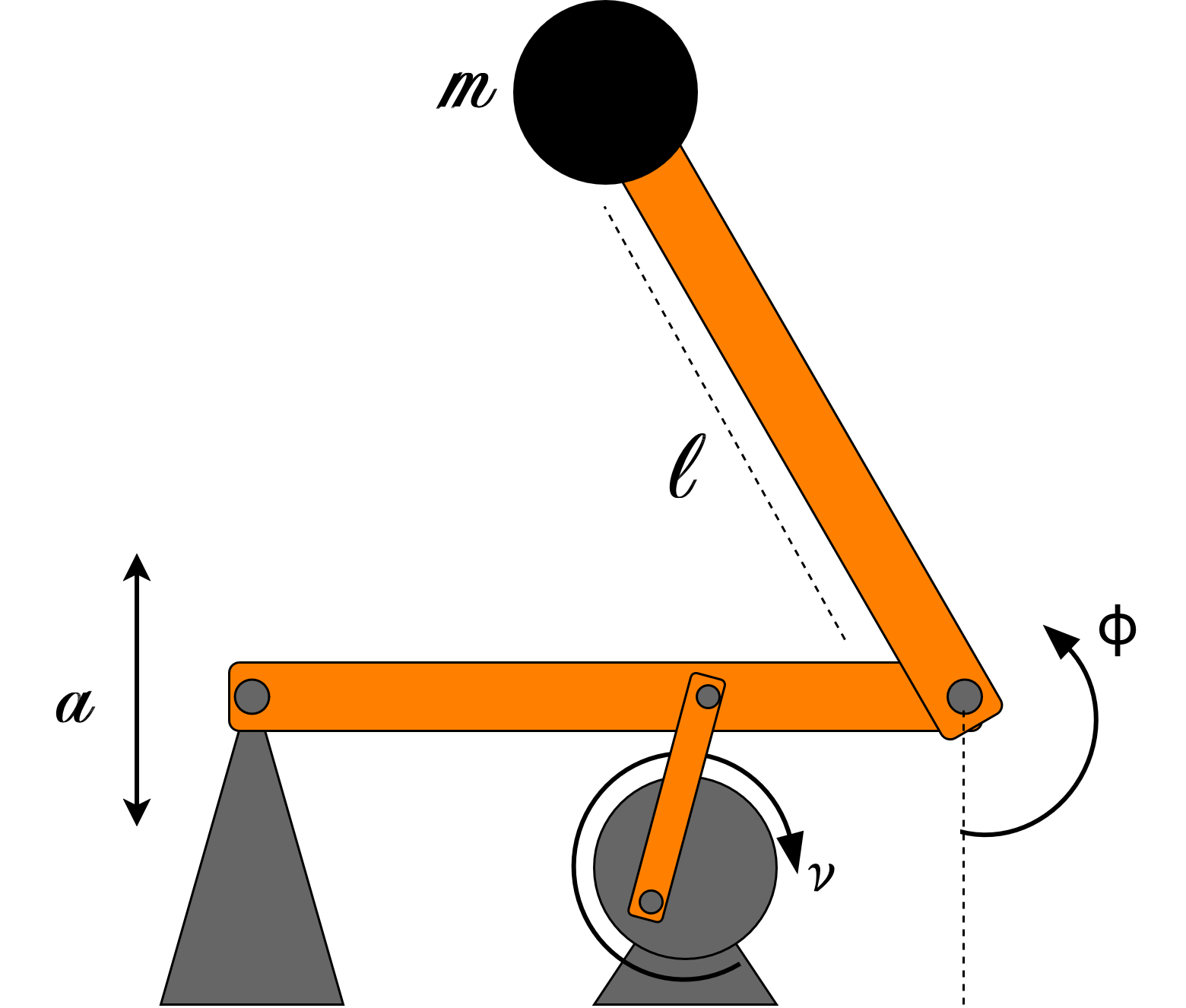
The Kapitza pendulum with driving frequency \(\nu\) and driving amplitude \(a\).
From this, we solve the Lagrangian: \[\mathcal{L} = \frac{1}{2}ml^2\dot{\phi}^2+mal\nu\dot{\phi}\sin{(\phi)}\sin{(\nu t)}+mgl\cos{(\phi)}\]
and attain the equation of motion \[\ddot{\phi} = -(g+a\nu^2 \cos{(\nu t)}) \frac{\sin{(\phi)}}{l}\]
Using a mix of analytical and numerical methods, we analyze when the vertical position of the pendulum is stable and when we have chaos through Hopf bifurcations. Specifically, we look at one specific functioning regime: the high-driving, low-amplitude regime. From analytical analysis, we can find the effective potential of this system, \[U_{\rm eff}(\phi) \approx -mgl\cos{(\phi)} + \frac{ma^2\nu^2}{4}\sin^2{(\phi)}\]
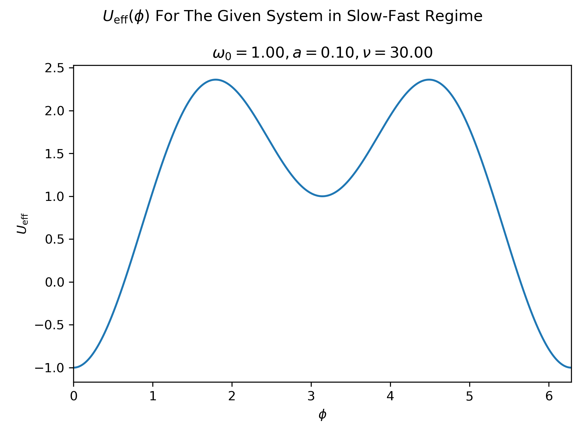
An example plot of \(U_{\rm eff}(\phi)\) for a natural frequency \(\omega_0=1\), \(a=1\) and \(\nu=30\).
We can see for this high-driving, low-amplitude regime, we can actually get a stable vertical position \(\phi=\pi\). Then, by doing bifurcation analysis on the system, we can fix the driving frequency and change the driving amplitude to identify when the vertical position is stable:
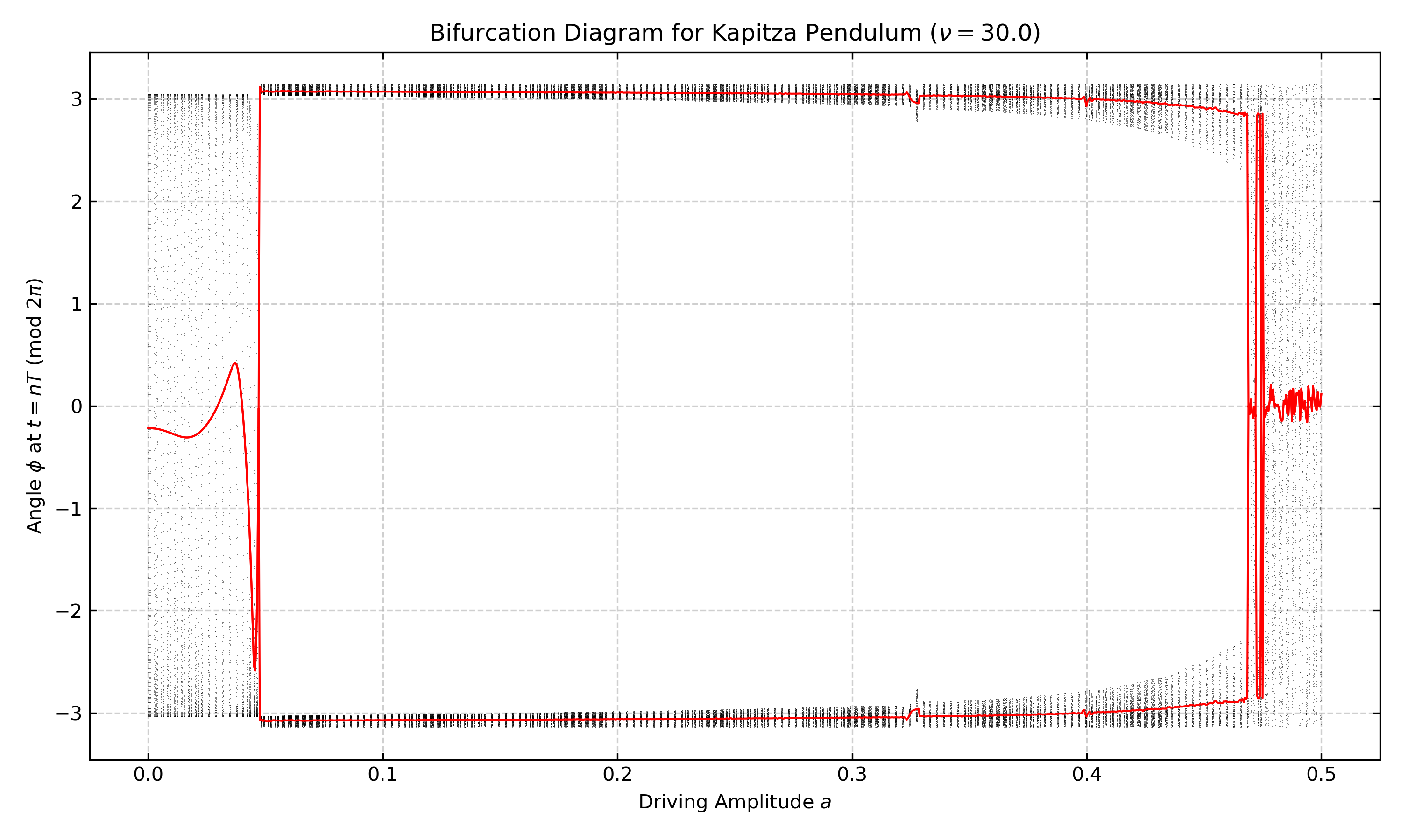
The Hopf bifurcation of the vertical position for \(\nu=30\).
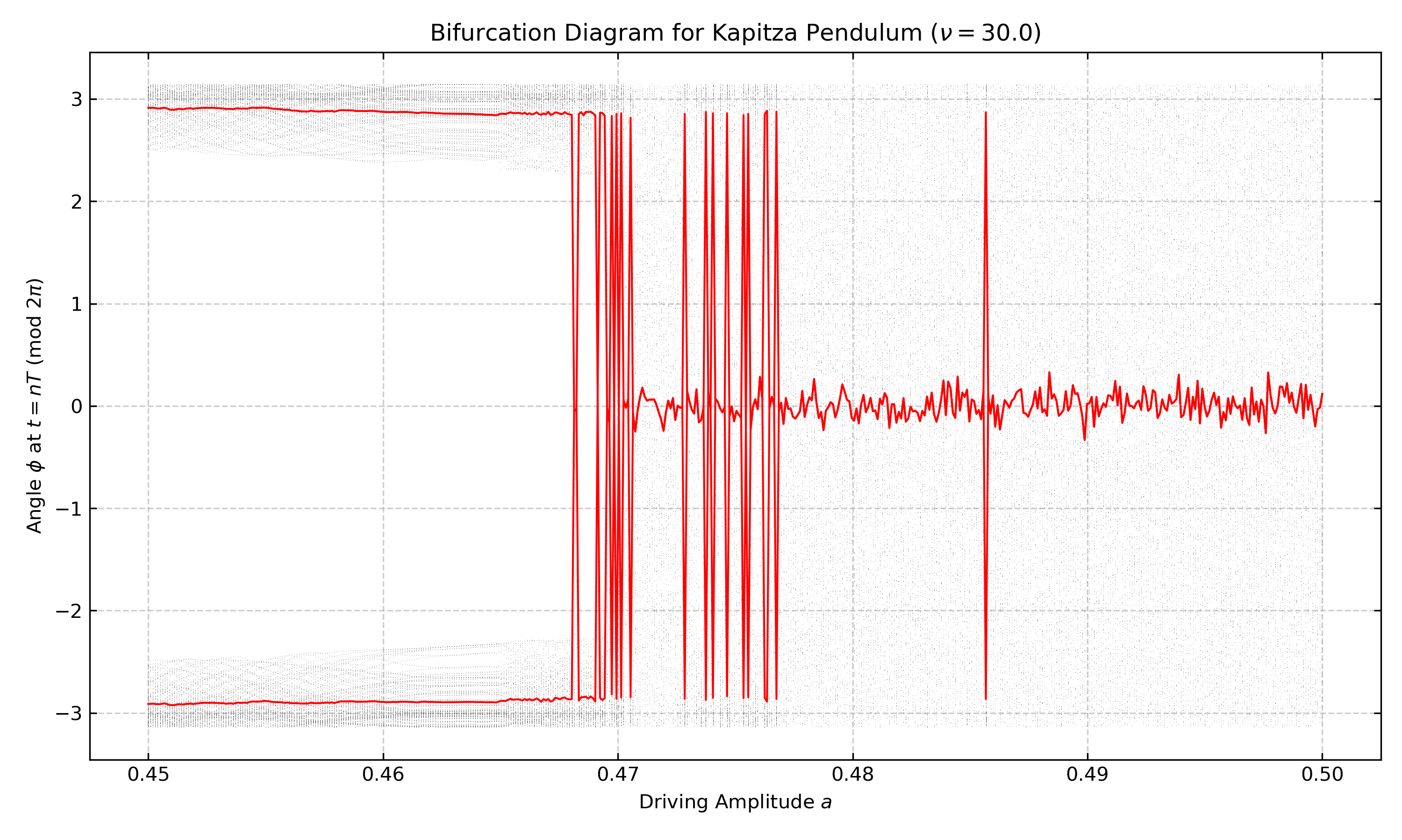
Same bifurcation for \(\nu=30\), investigating the right-hand area of the earlier plot.
From these analyses, we can find “windows” where the vertical position is stable, and locations where we expect chaotic motion.
More
This is a very high-level overview of this project. To get all the details, check the project file. If you’d like to learn more about the analytical results about the effective potentials and even the conditions for stability, check the derivation file on the slow-fast decomposition of motion. For a succinct overview that gives more background details, check the PDF of the presentation given for this project.
